import numpy as np
import matplotlib.pyplot as plt
import os
from pathlib import Path
from scipy.signal import convolve2dEvolution of Computer Vision
A Review of Traditional and Deep Learning Approaches
Origins
- It all started with CNNs
- Foundation of recent advances in computer vision
- Architectures based on this model have been the most successful in the field
Origins: Cat Neural Networks (CNNs)
I am obviously talking about Cat Neural Networks (this is a satirical point, not an inaccuracy in my presentation)
Receptive fields of single neurones in the cat’s striate cortex
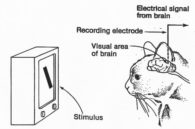
I dabble in neuroscience
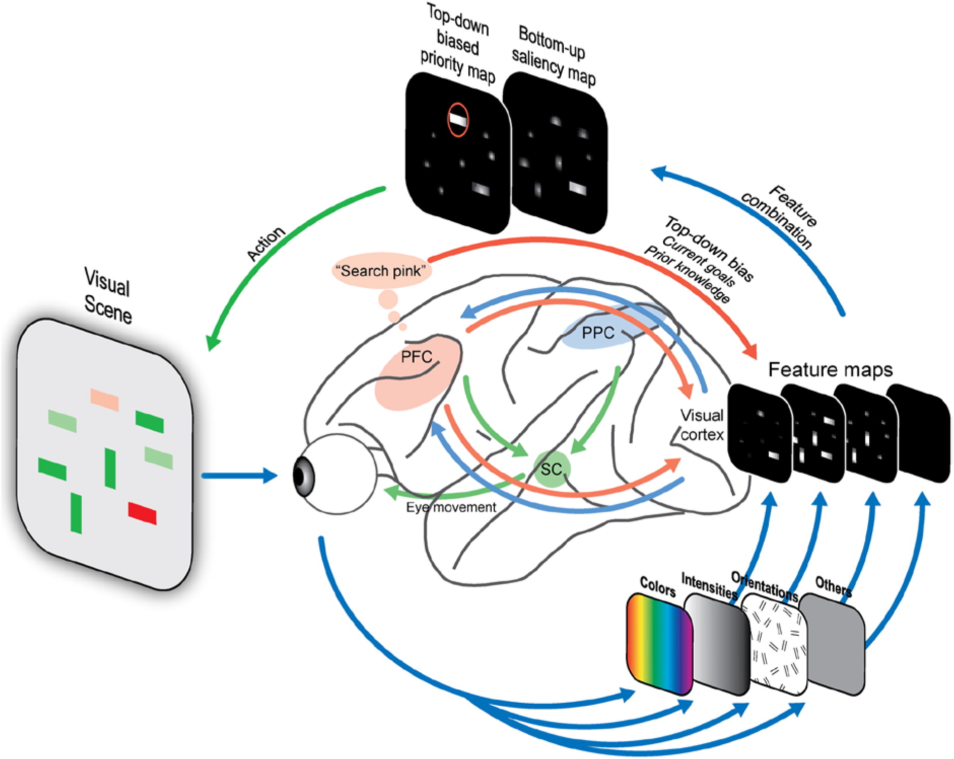
Psychology: Bottom-Up Processing
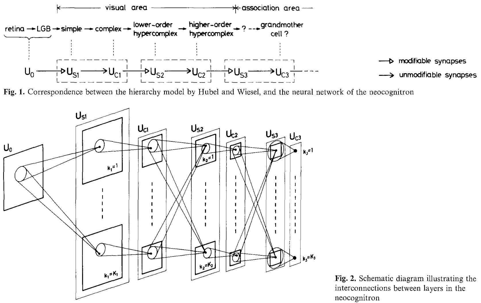
hierarchy structure : LGB (lateral geniculate body) -> simple cells -> complex cells -> lower order hypercomplex cells -> higher order hypercomplex cells
Neocognitron
neural networks to process images existed before, innovation is making it “deep” with convolutional layers basically first deep learning for CV
What are images?
img = plt.imread('images/bean.png')
gray_img = np.mean(img, axis=2)

fig, ax = plt.subplots(1, 2)
ax[0].imshow(img)
ax[1].imshow(gray_img, cmap='gray')
plt.show()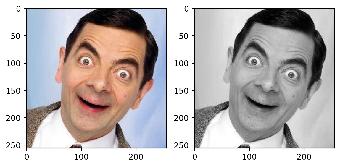
Images as Functions
def gaussian_kernel(size, sigma=1):
    size = int(size) // 2
    x, y = np.mgrid[-size:size+1, -size:size+1]
    normal = 1 / (2.0 * np.pi * sigma**2)
    g =  np.exp(-((x**2 + y**2) / (2.0*sigma**2))) * normal
    return g

kernel = gaussian_kernel(5, sigma=1)

blurred = convolve2d(gray_img, kernel, mode='same')

X = np.arange(gray_img.shape[0])
Y = np.arange(gray_img.shape[1])
X, Y = np.meshgrid(X, Y)
fig, ax = plt.subplots(subplot_kw={"projection": "3d"}); fig.set_size_inches(8, 7)
surf = ax.plot_surface(X, Y, 1 - np.flipud(blurred), cmap='summer')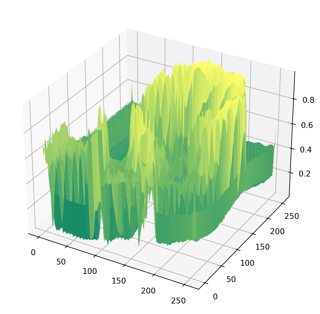
\(f\left(x,\ y\right)=\)
How to detect edges?
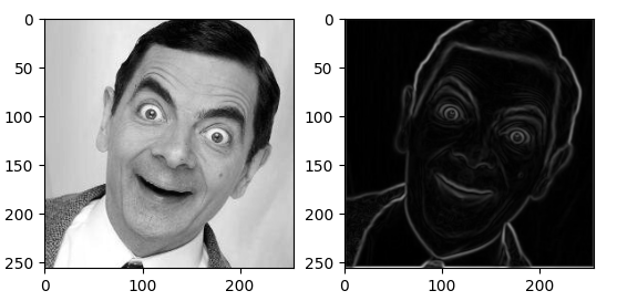
Gradients
- Steep cliffs where intensity changes rapidly
- Use some calculus
- \(\nabla f = \begin{bmatrix} \frac{\partial f}{\partial x} \\ \frac{\partial f}{\partial y} \end{bmatrix}\)
fig, ax = plt.subplots(1, 3); fig.set_figwidth(12)

bounded = gray_img.copy()
bounded[49:150, 49] = 0
bounded[49:150, 150] = 0
bounded[49, 49:150] = 0
bounded[150, 49:150] = 0

bounded_2 = gray_img.copy()
bounded_2[80:115, 85] = 0
bounded_2[80:115, 120] = 0
bounded_2[80, 85:120] = 0
bounded_2[115, 85:120] = 0

ax[0].imshow(bounded, cmap='gray')
ax[1].imshow(bounded_2[49:150, 49:150], cmap='gray')
ax[2].imshow(gray_img[80:115, 85:120], cmap='gray')
plt.show()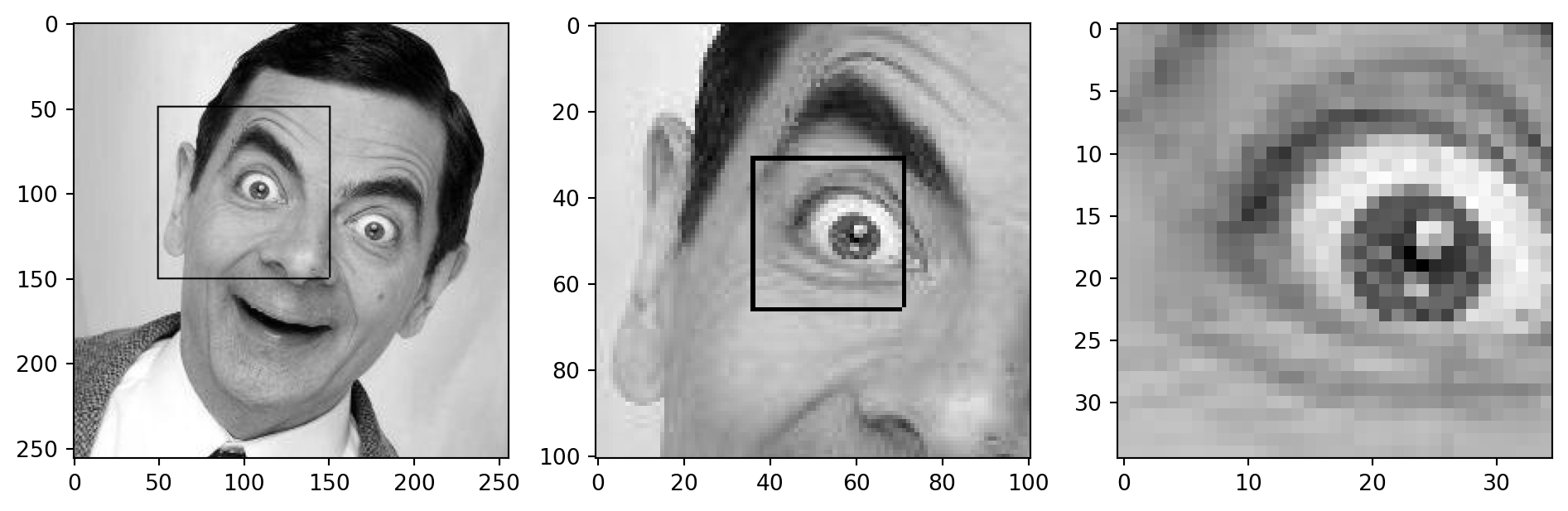
Convolution
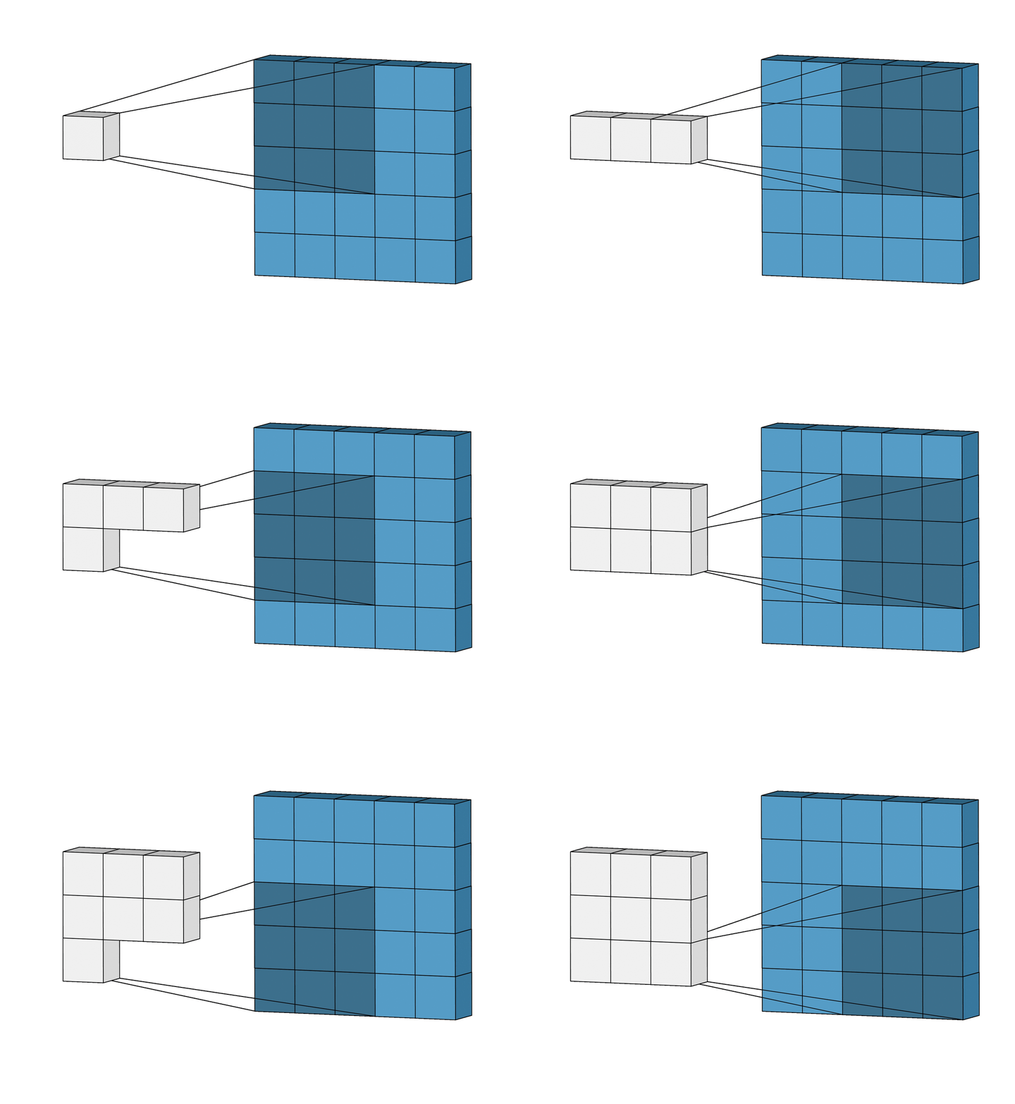
Convolution
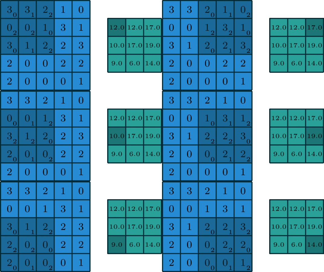
Sobel
sobel_x = np.array([[-1, 0, 1],
                    [-2, 0, 2],
                    [-1, 0, 1]])
# sobel operator for y-direction
sobel_y = np.array([[1, 2, 1],
                    [0, 0, 0],
                    [-1, -2, -1]])
Sobel Linear Filter
convolved_x = convolve2d(blurred, sobel_x, mode='same')
convolved_y = convolve2d(blurred, sobel_y, mode='same')
combined_edges = np.sqrt(convolved_x**2 + convolved_y**2)
fig, ax = plt.subplots(1, 3)
fig.set_figwidth(12)
ax[0].imshow(convolved_x, cmap='gray')
ax[0].set_title('Horizontal Edges', y=-0.25)
ax[1].imshow(convolved_y, cmap='gray')
ax[1].set_title('Vertical Edges', y=-0.25)
ax[2].imshow(combined_edges, cmap='gray')
ax[2].set_title('Norm Edges', y=-0.25)
plt.show()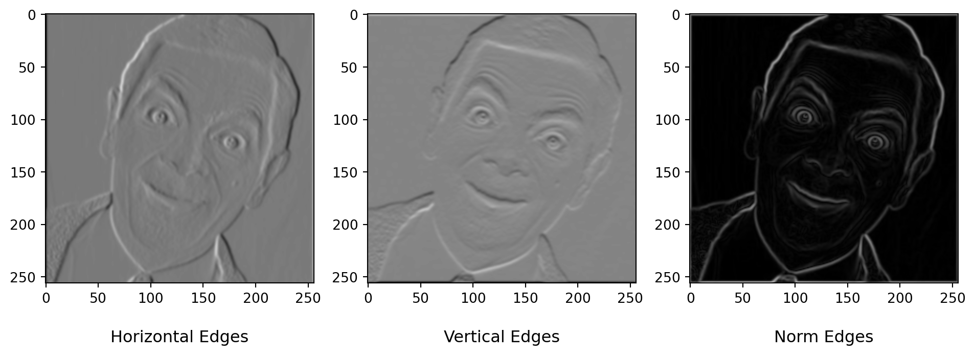
Other Filters
mean_kernel = np.ones((3, 3))

sharpen_kernel = np.array([[0, -1, 0],
                           [-1, 5, -1],
                           [0, -1, 0]])

impulse_kernel = np.array([[0, 0, 0],
                           [0, 1, 0],
                           [0, 0, 0]])

mean_blurred = convolve2d(gray_img, mean_kernel, mode='same')

sharpened = convolve2d(gray_img, sharpen_kernel, mode='same')
sharpened = np.clip(sharpened, 0, 1)

impulse = convolve2d(gray_img, impulse_kernel, mode='same')

fig, ax = plt.subplots(2, 3)
fig.set_size_inches(12, 7.5)
ax[0][0].imshow(mean_kernel, cmap='gray')
ax[0][0].set_title('Mean Kernel', y=-0.2)
ax[0][1].imshow(sharpen_kernel, cmap='gray')
ax[0][1].set_title('Sharpen Kernel', y=-0.2)
ax[0][2].imshow(impulse_kernel, cmap='gray')
ax[0][2].set_title('Impulse Kernel', y=-0.2)

kernels = [mean_kernel, sharpen_kernel, impulse_kernel]

for i in range(3):
  for r in range(3):
    for c in range(3):
      ax[0][i].text(c, r, kernels[i][r, c], ha="center", va="center", color="g", fontsize="large")

ax[1][0].imshow(mean_blurred / 9, cmap='gray')
ax[1][0].set_title('Mean Blur', y=-0.2)
ax[1][1].imshow(sharpened, cmap='gray')
ax[1][1].set_title('Sharpen', y=-0.2)
ax[1][2].imshow(impulse, cmap='gray')
ax[1][2].set_title('Impulse', y=-0.2)
plt.show()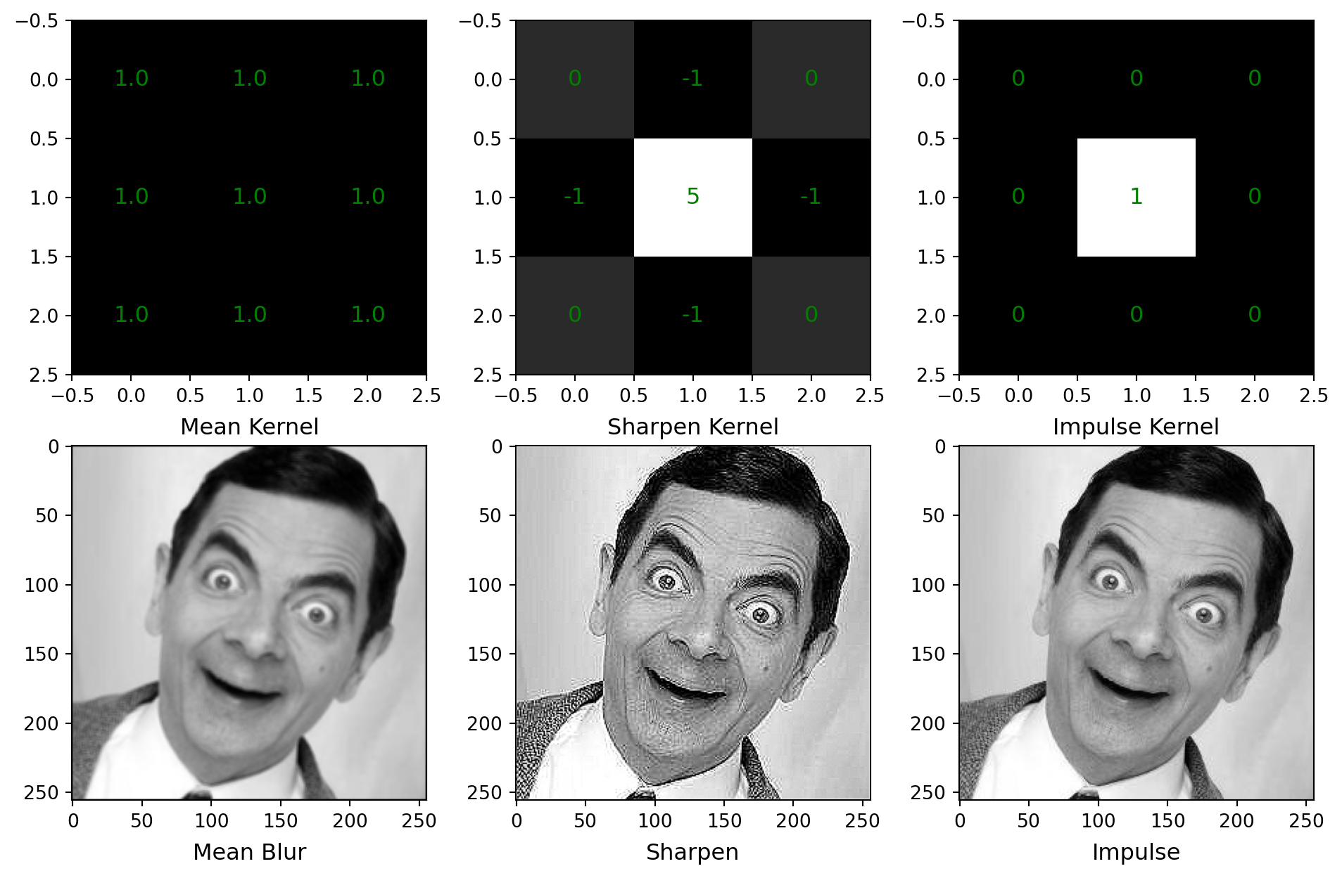
Traditional Computer Vision
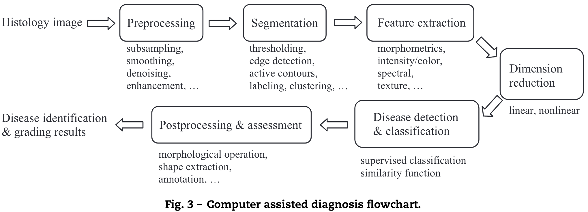
- Preprocessing: Denoising, Edge Detection, Subsampling
- Segmentation: Thresholding, Active Contours
- Feature Extraction: Scale Invariant Feature Transform (SIFT), Speeded Up Robust Features (SURF)
- Dimension Reduction: PCA
- Classification: Support Vector Machines (SVM), Random Forests, Boosting, Bagging, K-Nearest Neighbors (KNN)
Domain: Computer Aided Diagnosis
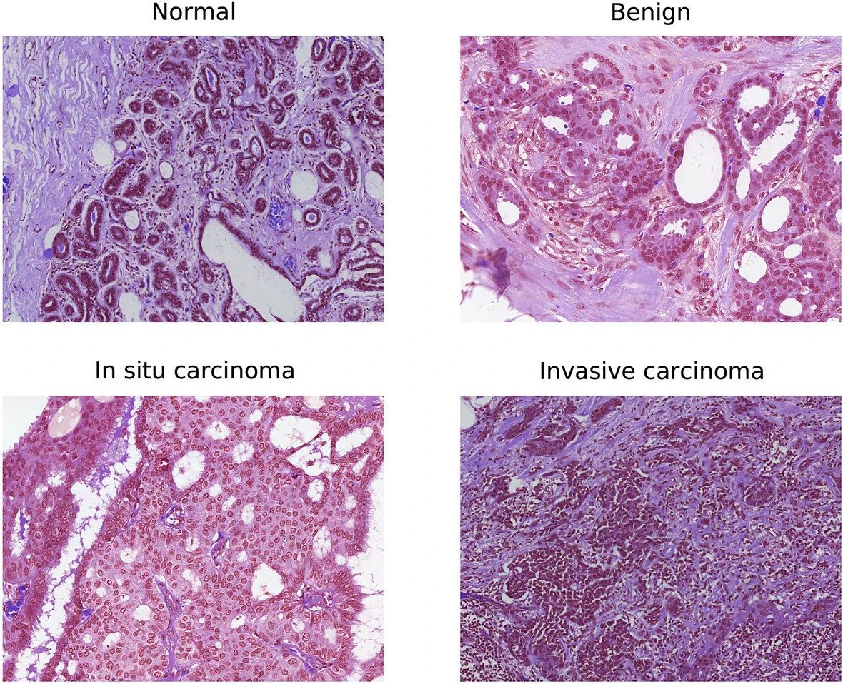
Diagnosis Pipeline
LeNet-5
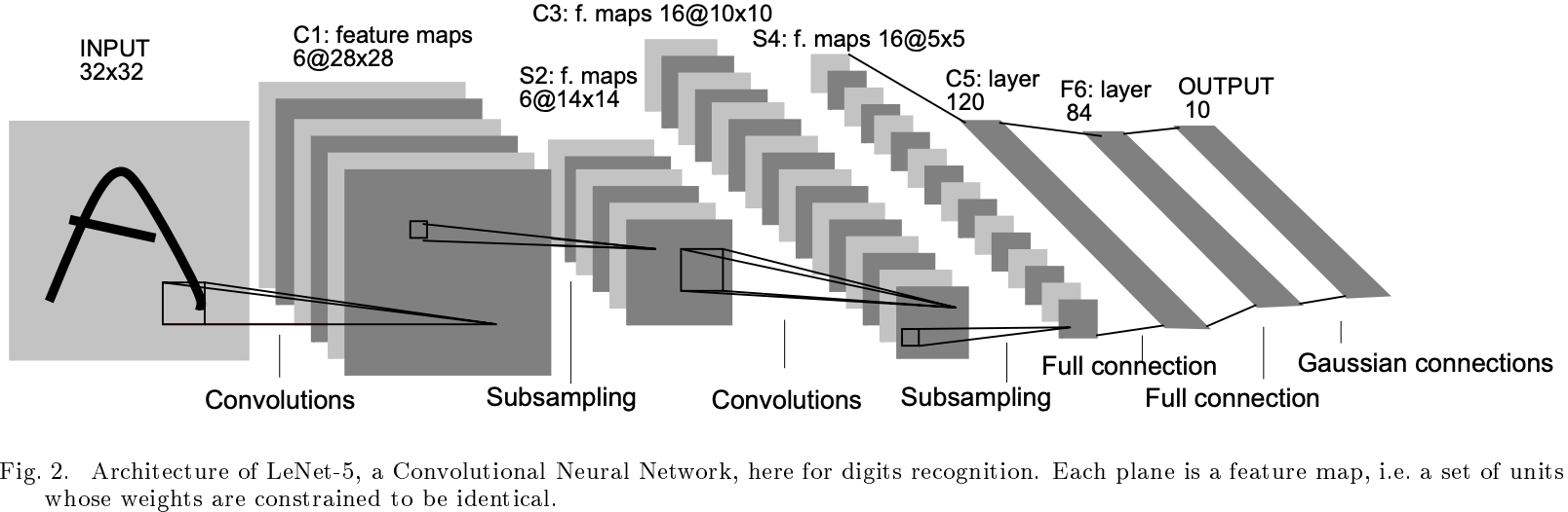
First Convolutional Neural Network as we know it today
Comparison
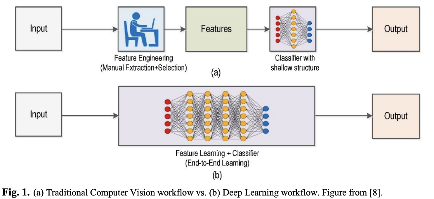
One Small Step
Limitations of the Past
- Lack of large structured datasets
- Lack of computational power
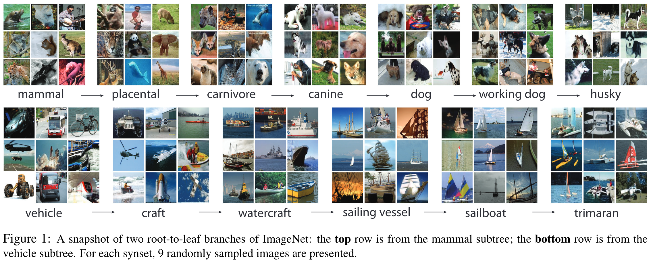
ImageNet: A Large-Scale Hierarchical Image Database
- 3.2 million images at time of publication
- PASCAL VOC
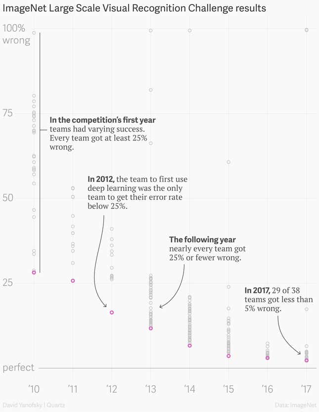
- ImageNet Large Scale Visual Recognition Challenge (ILSVRC)
Fei-Fei Li
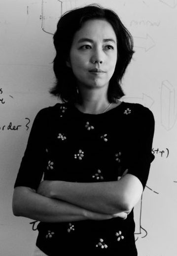
ImageNet: Snapshot
Breakthrough: AlexNet
- Imagenet has 15 million images at this point
- 1.2 million images used to train
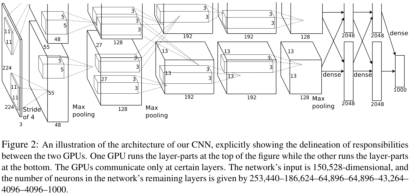
- 60 million parameters; 5 convolutional layers
- Cross-GPU parallelization (2x GTX 580)
- Non-saturating neurons (ReLU instead of tanh)
- Overfitting: Dropout, Data Augmentation (cropping, flipping, color shifting) (training size effectively x2048)
ImageNet Classification with Deep Convolutional Neural Networks: Architecture
Review
Traditional Techniques
- Tedious and time consuming
- Infeasible for complex images
- FAST
Deep Learning
- “Easy”
- LARGE datasets
- Expensive compute
Hybrid / Mixed Approaches
Rare cancer detection is hard
References
[1] Jia Deng, Wei Dong, Richard Socher, Li-Jia Li, Kai Li, and Li Fei-Fei. 2009. ImageNet: A large-scale hierarchical image database. In 2009 IEEE Conference on Computer Vision and Pattern Recognition, June 2009. 248–255. . https://doi.org/10.1109/CVPR.2009.5206848
[2] Kunihiko Fukushima. 1988. Neocognitron: A hierarchical neural network capable of visual pattern recognition. Neural Networks 1, 2 (January 1988), 119–130. https://doi.org/10.1016/0893-6080(88)90014-7
[3] Zabit Hameed, Begonya Garcia-Zapirain, José Javier Aguirre, and Mario Arturo Isaza-Ruget. 2022. Multiclass classification of breast cancer histopathology images using multilevel features of deep convolutional neural network. Sci Rep 12, 1 (September 2022), 15600. https://doi.org/10.1038/s41598-022-19278-2
[4] Lei He, L. Rodney Long, Sameer Antani, and George R. Thoma. 2012. Histology image analysis for carcinoma detection and grading. Computer Methods and Programs in Biomedicine 107, 3 (September 2012), 538–556. https://doi.org/10.1016/j.cmpb.2011.12.007
[5] D. H. Hubel and T. N. Wiesel. 1959. Receptive fields of single neurones in the cat’s striate cortex. J Physiol 148, 3 (October 1959), 574–591.
[6] Fumi Katsuki and Christos Constantinidis. 2014. Bottom-Up and Top-Down Attention: Different Processes and Overlapping Neural Systems. Neuroscientist 20, 5 (October 2014), 509–521. https://doi.org/10.1177/1073858413514136
[7] Alex Krizhevsky, Ilya Sutskever, and Geoffrey E Hinton. 2012. ImageNet Classification with Deep Convolutional Neural Networks. In Advances in Neural Information Processing Systems, 2012. Curran Associates, Inc. . Retrieved December 1, 2023 from https://papers.nips.cc/paper_files/paper/2012/hash/c399862d3b9d6b76c8436e924a68c45b-Abstract.html
[8] Brajesh Kumar. 2021. Convolutional Neural Networks: A Brief History of their Evolution. AppyHigh Blog. Retrieved December 1, 2023 from https://medium.com/appyhigh-technology-blog/convolutional-neural-networks-a-brief-history-of-their-evolution-ee3405568597
[9] Yann LeCun, Leon Bottou, Yoshua Bengio, and Patrick Ha. 1998. Gradient-Based Learning Applied to Document Recognition. (1998).
[10] Niall O’ Mahony, Sean Campbell, Anderson Carvalho, Suman Harapanahalli, Gustavo Velasco-Hernandez, Lenka Krpalkova, Daniel Riordan, and Joseph Walsh. 2020. Deep Learning vs. Traditional Computer Vision. https://doi.org/10.1007/978-3-030-17795-9
[11] Irhum Shafkat. 2018. Intuitively Understanding Convolutions for Deep Learning. Medium. Retrieved December 3, 2023 from https://towardsdatascience.com/intuitively-understanding-convolutions-for-deep-learning-1f6f42faee1
[12] Richard Szeliski. 2022. Computer Vision: Algorithms and Applications. Springer International Publishing, Cham. https://doi.org/10.1007/978-3-030-34372-9
[13] Xiongwei Wu, Doyen Sahoo, and Steven C. H. Hoi. 2020. Recent advances in deep learning for object detection. Neurocomputing 396, (July 2020), 39–64. https://doi.org/10.1016/j.neucom.2020.01.085
[14] 2017. The data that transformed AI research—and possibly the world. Quartz. Retrieved December 1, 2023 from https://qz.com/1034972/the-data-that-changed-the-direction-of-ai-research-and-possibly-the-world
[15] A Brief History of Computer Vision (and Convolutional Neural Networks) | HackerNoon. Retrieved December 1, 2023 from https://hackernoon.com/a-brief-history-of-computer-vision-and-convolutional-neural-networks-8fe8aacc79f3
[16] CS5670: Introduction to Computer Vision, Spring 2023 – Cornell Tech. Retrieved December 2, 2023 from https://www.cs.cornell.edu/courses/cs5670/2023sp/